Correspondence Analysis

Concept: Correspondence Analysis

Core Intuition

Correspondence Analysis (CA) is a dimensionality reduction and data visualization technique for contingency tables of counts. It reveals associations between row and column categories by mapping them into a shared low-dimensional space, where proximity indicates similarity of profiles.

Three key properties:

• Aggregate data based: operates on summarized count tables, not raw observations.
• Dimension reduction: represents associations in a table of nonnegative counts.
• Data visualization for association: positions of points reflect category associations.

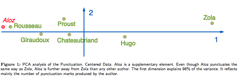
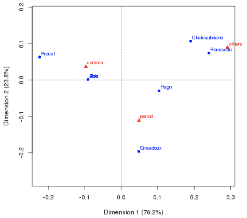
Why not PCA? PCA is sensitive to the magnitude of counts, not their relative profiles. In the French authors dataset (punctuation style by author), PCA places Aloz far from Zola despite identical punctuation style — because Aloz wrote a short novel. CA normalizes by profile, correctly grouping Aloz and Zola together.

Example applications

• Segments vs. genders / hours / weekdays / locations / app detection
• Segments vs. {only-impressions, with-clicks, with-actions}
• Campaigns vs. {only-impressions, with-clicks, with-actions}
• Other groups vs. characteristics, etc.

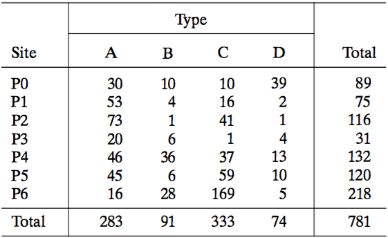
Archaeological example: sites vs. types

Common bar charts cannot quantify associations:

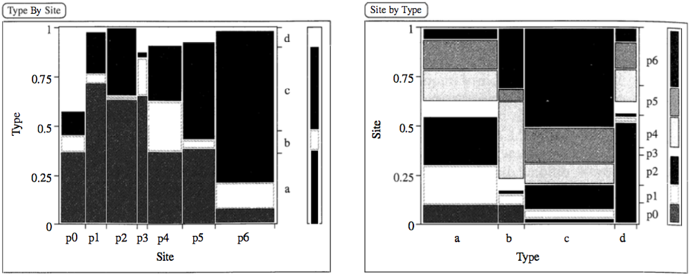
CA visualization:

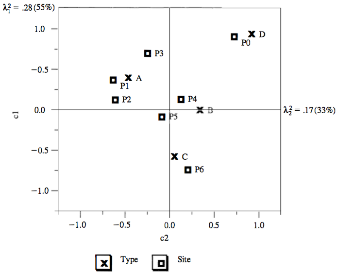
• Sites association:
  • P1 and P2 are close together, thus have similar type profiles
  • P0 and P6 are far apart, thus have different type profiles
• Types association:
  • A, B, C and D have different site profiles
• Site and type association: (rough, see later)
  • Site P0 is associated almost exclusively with type D
  • Site P6 is similarly associated with type C
  • Sites P1, P2 and P3 (to lesser degrees) are associated with type A
• Measure of retained information:
  • Inertia: amount of retained information with
    • 1st dimension: ${\lambda }_1^2=0.28(55\%)$
    • 2nd dimension: ${\lambda }_2^2=0.17(28\%)$
  • The two dimensions account for $55\%+28\%=88\%$ of the total inertia
  • The representation fits the data well

Mathematical Foundation

CA is based on generalized singular value decomposition (SVD), similar to PCA, except it applies to categorical rather than continuous data.

Setup

Let the observed data be a contingency table of unscaled counts:

$$\underset{(I\times J)}{X}=\{x_{ij}\}=\left[\begin{array}{ccc}{x}_{11}& \cdots & x_{1J}\\ ⋮& & ⋮\\ x_{I1}& \cdots & x_{IJ}\end{array}\right]$$

The rows and columns of $X$ correspond to different categories (groups) of different characteristics.

Correspondence Matrix and Profiles

Correspondence matrix: divide $x_{ij}$ by total count $n={\sum }_{i=1}^I{\sum }_{j=1}^J{x}_{ij}$:

$$p_{ij}=\frac{1}{n}{x}_{ij},\underset{I\times J}{P}=\frac{1}{n}X$$

Row and column marginal profiles:

$$r_i=\sum _{j=1}^J{p}_{ij}=\frac{1}{n}\sum _{j=1}^J{x}_{ij},\underset{I\times 1}{r}=P{1}_J$$ $$c_j=\sum _{i=1}^I{p}_{ij}=\frac{1}{n}\sum _{i=1}^I{x}_{ij},\underset{J\times 1}{c}=P^T{1}_I$$

Diagonal weight matrices:

$$D_r=\text{diag}(r_1,\dots ,r_I)$$ $$D_c=\text{diag}(c_1,\dots ,c_J)$$

Weighted Least Squares Formulation

CA finds a reduced rank-$K$ approximation $\hat{P}=\{{\hat{p}}_{ij}\}$ minimizing:

$$\sum _{i=1}^I\sum _{j=1}^J\frac{{\left(p_{ij}-{\hat{p}}_{ij}\right)}^2}{r_i{c}_j}=\text{tr}\left[\left(D_r^{-1/2}(P-\hat{P})D_c^{-1/2}\right){\left(D_r^{-1/2}(P-\hat{P})D_c^{-1/2}\right)}^T\right]$$

Result from (Johnson & Wichern, 2002, p. 72): The term $r{c}^T$ is common to the approximation $\hat{P}$ whatever the correspondence matrix $P$. Thus it is equivalent to minimize:

$$\text{tr}\left[\left(D_r^{-1/2}(P-r{c}^T-\hat{P})D_c^{-1/2}\right){\left(D_r^{-1/2}(P-r{c}^T-\hat{P})D_c^{-1/2}\right)}^T\right]$$

Generalized SVD

Compute the SVD of $D_r^{-1/2}(P-r{c}^T)D_c^{-1/2}$:

$$D_r^{-1/2}(P-r{c}^T)D_c^{-1/2}=U\Sigma V^T$$

where $U$ and $V$ are orthogonal matrices with $U^{T}U=V^{T}V=I$, and $\Sigma$ is a rank-$K$ diagonal matrix. Thus:

$$P-r{c}^T=D_r^{1/2}\left(U\Sigma V^T\right)D_c^{1/2}=A\Sigma B^T$$

where $A=D_r^{1/2}U$ and $B=D_c^{1/2}V$. This decomposition is called the generalized SVD:

$$P-r{c}^T=A\Sigma B^T,\text{with }{A}^T{D}_r^{-1}A=B^T{D}_c^{-1}B=I$$

Row and Column Profile Matrices

Row profile matrix (divide each row by its sum):

$$R=D_r^{-1}P=\left[\begin{array}{cccc}\frac{p_{11}}{r_1}& \frac{p_{12}}{r_1}& \cdots & \frac{p_{1J}}{r_1}\\ ⋮& & & ⋮\\ \frac{p_{I1}}{r_I}& \frac{p_{I2}}{r_I}& \cdots & \frac{p_{IJ}}{r_I}\end{array}\right]$$

Column profile matrix (divide each column by its sum):

$$C=P{D}_c^{-1}=\left[\begin{array}{cccc}\frac{p_{11}}{c_1}& \frac{p_{12}}{c_2}& \cdots & \frac{p_{1J}}{c_J}\\ ⋮& & & ⋮\\ \frac{p_{I1}}{c_1}& \frac{p_{I2}}{c_2}& \cdots & \frac{p_{IJ}}{c_J}\end{array}\right]$$

Row deviations from average row profile:

$$R-1_I{c}^T=D_r^{-1}P-1_I{c}^T=D_r^{-1}(P-r{c}^T)=D_r^{-1}A\Sigma B^T=D_r^{-1}\left(D_r^{1/2}U\right)\Sigma B^T=D_r^{-1/2}U\Sigma B^T$$

Column deviations from average column profile: similarly,

$$(C-r{1}_J^T{)}^T=D_c^{-1}P-r{1}_J^T=D_c^{-1/2}V\Sigma A^T$$

Principal and Standard Coordinates

Hence, we can obtain coordinates of the row and column profiles:

Principal coordinates of rows: the coordinates for $(R-1_I{c}^T)$ w.r.t. the axes of $b_1,\dots ,b_J$ are given by the columns of

$$F=D_r^{-1/2}U\Sigma$$

Principal coordinates of columns: the coordinates for $(C-r{1}_J^T{)}^T$ w.r.t. the axes of $a_1,\dots ,a_I$ are given by the columns of

$$G=D_c^{-1/2}V\Sigma$$

Standard coordinates of rows:

$$\Phi =D_r^{-1/2}U$$

Standard coordinates of columns:

$$\Gamma =D_c^{-1/2}V$$

Relationships:

$$F^T{D}_{r}F=G^T{D}_{c}G={\Sigma }^2$$ $${\Phi }^T{D}_r\Phi ={\Gamma }^T{D}_c\Gamma =I$$

Inertia

Total variance of the correspondence matrix $P$, resembling a chi-square statistic:

$$\text{Inertia}=\sum _{i=1}^I\sum _{j=1}^J\frac{{\left(p_{ij}-r_i{c}_j\right)}^2}{r_i{c}_j}=\sum _{k=1}^K{\lambda }_k^2$$

Evaluation of 2D graphical display:

• Inertia associated with dimension $k$, for $k=1,2$: ${\lambda }_k^2$.
• Proportion of total inertia: explained total variance; the larger, the better.

$$\frac{\left({\lambda }_1^2+{\lambda }_2^2\right)}{{\sum }_{k=1}^K{\lambda }_k^2}$$

Visualization Maps

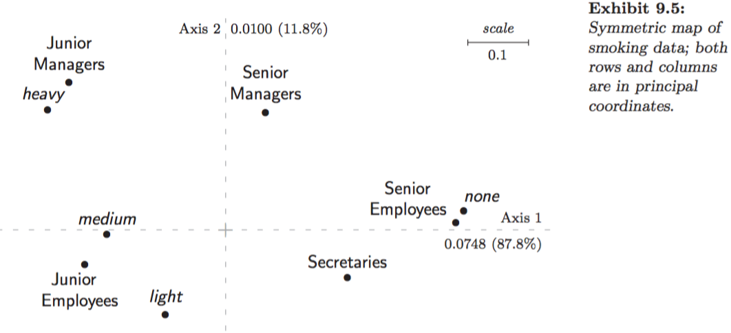
• (1) Symmetric map: $(F,G)$, rows and columns in principal coordinates.
• (2) Asymmetric map with row principal: $(F,\Gamma )$, rows (of more interest) in principal and columns in standard coordinates.
• (3) Asymmetric map with column principal: $(\Phi ,G)$, rows in standard and columns (of more interest) in principal coordinates.

For interpretation details see (Greenacre, 2007, p. 66-72).

Symmetric map (1):

• Since principal coordinates $(F,G)$ are scaled similarly, joint display of two separate maps finds some justification.
• Thus, row-to-row and column-to-column distance interpretations are meaningful.
• However, there is a danger in row-to-column distance interpretation: not possible to deduce from the closeness of a row and column point that the corresponding row and column necessarily have a high association, since the row space and column space are different.

Asymmetric maps (2) and (3):

• The row and column points lie in the same space (since $F$ is with respect to basis $B$, and $\Gamma B^T=I$), thus not only row-to-row and column-to-column distance interpretations, but also row-to-column distance interpretation are meaningful.
• Closeness of a row and column point indicates a high association; row-to-column distances can be calculated one column at a time.

Interpretations:

• Asymmetric plots allow intuitively interpreting row-to-row, column-to-column, and row-to-column distances, especially when the first two components have a large proportion of total inertia.
• However, principal points on an asymmetric plot might appear too close to each other in the center of the map. In that case, also display a symmetric plot to more clearly view the relationships among either the row or column categories.

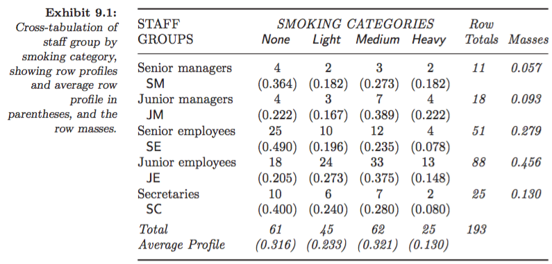
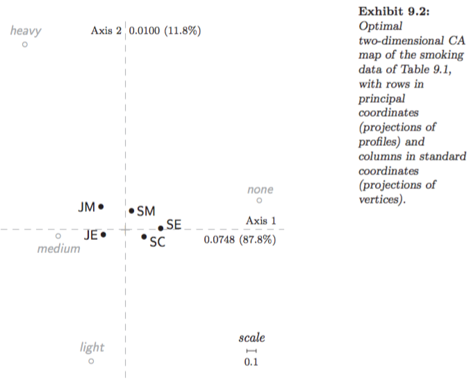
Example: Smoking dataset:

Asymmetric map, row principal (Greenacre 2007, Fig. 9.2):

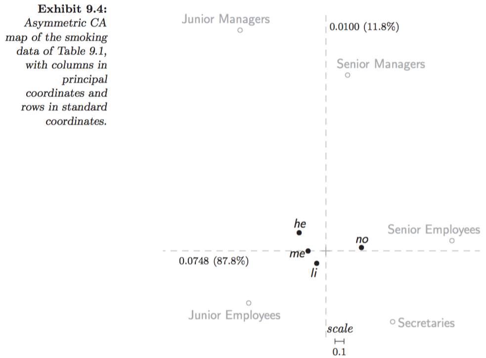
Asymmetric map, column principal (Greenacre 2007, Fig. 9.4):

Symmetric map (Greenacre 2007, Fig. 9.5):

French Authors Dataset

Goal: derive a map that reveals the similarities in punctuation style between authors. Note: Zola wrote a short novel under the pseudonym Aloz.

import numpy as np
import scipy as sp
import pandas as pd
 
data = {'period': [7836, 53655, 115615, 161926, 38177, 46371, 2699],
        'comma':  [13112, 102383, 184541, 340479, 105101, 58367, 5675],
        'others': [6026, 42413, 59226, 62754, 12670, 14299, 1046]}
data = pd.DataFrame(data, columns=['period', 'comma', 'others'],
                    index=['Rousseau', 'Chateaubriand', 'Hugo',
                           'Zola', 'Proust', 'Giraudoux', 'Aloz'])

	period	comma	others
Rousseau	7836	13112	6026
Chateaubriand	53655	102383	42413
Hugo	115615	184541	59226
Zola	161926	340479	62754
Proust	38177	105101	12670
Giraudoux	46371	58367	14299
Aloz	2699	5675	1046

Key Equation

$$D_r^{-1/2}(P-r{c}^T)D_c^{-1/2}=U\Sigma V^T\text{(generalized SVD)}$$ $$F=D_r^{-1/2}U\Sigma ,G=D_c^{-1/2}V\Sigma \text{(principal coordinates)}$$ $$\text{Inertia}=\sum _{k=1}^K{\lambda }_k^2\text{(total variance)}$$

Analogy

CA is PCA applied to a normalized residual table: instead of centering by subtracting the mean, it centers by subtracting the independence model $r{c}^T$, and instead of unit weighting it uses $D_r^{-1/2}$ and $D_c^{-1/2}$ to weight by marginal frequency — making profiles, not counts, the object of study.

Component of

• Dimensionality Reduction todo
• Exploratory Data Analysis todo

Insights

• CA operates on profiles (relative frequencies), making it invariant to overall count magnitude — this is why it correctly identifies Aloz as stylistically similar to Zola.
• The generalized SVD of $D_r^{-1/2}(P-r{c}^T)D_c^{-1/2}$ is the core computation; all coordinates follow from $U$, $V$, $\Sigma$.
• Inertia is a chi-square-like statistic: it measures total departure from independence.
• For interpretation, prefer asymmetric maps when row-to-column distances matter; use symmetric maps when within-group distances are the focus.

Pitfalls

• Symmetric maps tempt row-to-column distance interpretation, which is not geometrically valid.
• CA assumes the association structure is low-rank; if associations are diffuse, the 2D display retains little inertia and is misleading.
• CA is for count data; applying it to continuous measurements or negative values is inappropriate.

Connections

• PCA and SVD: CA is generalized SVD applied to the standardized residual of a correspondence matrix; PCA is ordinary SVD applied to continuous data.
• Generalized SVD todo
• Chi-Square Statistic todo

Implementation Notes

# https://github.com/bowen0701/machine-learning/blob/master/correspondence_analysis.py
import numpy as np
import pandas as pd
from numpy.linalg import svd
 
class CorrespondenceAnalysis(object):
    """Correspondence analysis (CA).
 
    Methods:
      fit: Fit correspondence analysis.
      get_coordinates: Get symmetric or asymmetric map coordinates.
      score_inertia: Get score inertia.
 
    Usage:
      corranal = CorrespondenceAnalysis(aggregate_cnt)
      corranal.fit()
      coord_df = corranal.get_coordinates()
      inertia_prop = corranal.score_inertia()
    """
 
    def __init__(self, df):
        """Create a new Correspondence Analysis.
 
        Args:
          df: Pandas DataFrame, with row and column names.
 
        Raises:
          TypeError: Input data is not a pandas DataFrame.
          ValueError: Input data contains missing values.
          TypeError: Input data contains data types other than numeric.
        """
        if not isinstance(df, pd.DataFrame):
            raise TypeError('Input data is not a Pandas DataFrame.')
        self._rows = np.array(df.index)
        self._cols = np.array(df.columns)
        self._np_data = np.array(df.values)
        if np.isnan(self._np_data).any():
            raise ValueError('Input data contains missing values.')
        if not np.issubdtype(self._np_data.dtype, np.number):
            raise TypeError('Input data contains data types other than numeric.')
 
    def fit(self):
        """Compute Correspondence Analysis.
 
        Performs generalized SVD for the correspondence matrix and
        computes principal and standard coordinates for rows and columns.
 
        Returns:
          self: Object.
        """
        p_corrmat = self._np_data / self._np_data.sum()
        r_profile = p_corrmat.sum(axis=1).reshape(p_corrmat.shape[0], 1)
        c_profile = p_corrmat.sum(axis=0).reshape(p_corrmat.shape[1], 1)
        Dr_invsqrt = np.diag(np.power(r_profile, -1/2).T[0])
        Dc_invsqrt = np.diag(np.power(c_profile, -1/2).T[0])
        ker_mat = np.subtract(p_corrmat, np.dot(r_profile, c_profile.T))
        weighted_lse = Dr_invsqrt.dot(ker_mat).dot(Dc_invsqrt)
        U, sv, Vt = svd(weighted_lse, full_matrices=False)
        self._Dr_invsqrt = Dr_invsqrt
        self._Dc_invsqrt = Dc_invsqrt
        self._U = U
        self._V = Vt.T
        self._SV = np.diag(sv)
        self._inertia = np.power(sv, 2)
        # Principal coordinates for rows and columns.
        self._F = self._Dr_invsqrt.dot(self._U).dot(self._SV)
        self._G = self._Dc_invsqrt.dot(self._V).dot(self._SV)
        # Standard coordinates for rows and columns.
        self._Phi = self._Dr_invsqrt.dot(self._U)
        self._Gam = self._Dc_invsqrt.dot(self._V)
        return self
 
    def _coordinates_df(self, array_x1, array_x2):
        """Create pandas DataFrame with coordinates in rows and columns.
 
        Args:
          array_x1: numpy array, coordinates in rows.
          array_x2: numpy array, coordinates in columns.
 
        Returns:
          coord_df: A Pandas DataFrame with columns
            {'x_1',..., 'x_K', 'point', 'coord'}:
            - x_k, k=1,...,K: K-dimensional coordinates.
            - point: row and column points for labeling.
            - coord: {'row', 'col'}, indicates row point or column point.
        """
        row_df = pd.DataFrame(
            array_x1,
            columns=['x' + str(i) for i in (np.arange(array_x1.shape[1]) + 1)])
        row_df['point'] = self._rows
        row_df['coord'] = 'row'
        col_df = pd.DataFrame(
            array_x2,
            columns=['x' + str(i) for i in (np.arange(array_x2.shape[1]) + 1)])
        col_df['point'] = self._cols
        col_df['coord'] = 'col'
        coord_df = pd.concat([row_df, col_df], ignore_index=True)
        return coord_df
 
    def get_coordinates(self, option='symmetric'):
        """Take coordinates in rows and columns for symmetric or asymmetric map.
 
        For symmetric vs. asymmetric map:
          - For symmetric map, we can catch row-to-row and column-to-column
            association (maybe not row-to-column association);
          - For asymmetric map, we can further catch row-to-column association.
 
        Args:
          option: string, one of:
            'symmetric': symmetric map with rows and columns in principal coordinates.
            'rowprincipal': asymmetric map with rows in principal coordinates and
              columns in standard coordinates.
            'colprincipal': asymmetric map with rows in standard coordinates and
              columns in principal coordinates.
 
        Returns:
          Pandas DataFrame, contains coordinates, row and column points.
 
        Raises:
          ValueError: Option only includes {"symmetric", "rowprincipal", "colprincipal"}.
        """
        if option == 'symmetric':
            return self._coordinates_df(self._F, self._G)
        elif option == 'rowprincipal':
            return self._coordinates_df(self._F, self._Gam)
        elif option == 'colprincipal':
            return self._coordinates_df(self._Phi, self._G)
        else:
            raise ValueError(
                'Option only includes {"symmetric", "rowprincipal", "colprincipal"}.')
 
    def score_inertia(self):
        """Score inertia.
 
        Returns:
          A NumPy array, contains proportions of total inertia explained
            in coordinate dimensions.
        """
        inertia = self._inertia
        inertia_prop = (inertia / inertia.sum()).cumsum()
        return inertia_prop

References

[1] Johnson & Wichern (2002). Applied Multivariate Statistical Analysis. [2] Nenadic & Greenacre (JSS, 2007). Correspondence Analysis in R, with Two- and Three-dimensional Graphics: The ca Package. [3] Greenacre (2007). Correspondence Analysis in Practice. [4] Greenacre (2010). Biplots in Practice.