PCA and SVD

Table of Contents

• Core Intuition
• Mathematical Foundation
  • Setup
  • PCA Assumptions
  • Eigendecomposition
  • SVD
  • Matrix Version of SVD
  • Connection Between PCA and SVD
  • How Many Principal Components to Use
  • Reduced Rank Approximation by SVD
  • PCA Algorithm Summary
• Key Equation
• Analogy
• Component of
• Insights
• Pitfalls
• Connections
• Implementation Notes
• References

Core Intuition

PCA identifies the most meaningful basis to re-express data by maximizing the signal-to-noise ratio (SNR): $\sigma^2{\text{signal}} / \sigma^2{\text{noise}}$ (Shlens 2014).

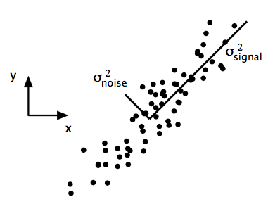
• Maximize signal: measured by variance magnitude; large variance encodes interesting structure.
• Minimize redundancy (noise): measured by covariance magnitude.

Mathematical Foundation

Setup

Let the observed data be

\[\underset{(m \times n)}X = \{x_{ij}\} = \begin{bmatrix} x_{11} & \cdots & x_{1n} \\ \vdots & & \vdots \\ x_{m1} & \cdots & x_{mn} \end{bmatrix} = \begin{bmatrix} x^T_{1.} \\ \vdots \\ x^T_{m.} \end{bmatrix} = [x_{.1}, \cdots, x_{.n}]\]

where each row $x^T_{i.}$ represents an example on $n$-dimensional features:

\[x^T_{i.} = [x_{i1} \dots x_{in}]\]

For notation simplicity, we also denote each row $x^T_{i.}$ by $x^T_i$. Each column

\[x_{.j}= \begin{bmatrix} x_{1j} \\ \vdots \\ x_{mj} \end{bmatrix}\]

is normalized to zero mean $E(x_{.j}) = 0$ and unit variance $\text{Var}(x_{.j}) = 1$ (Johnson & Wichern 2002).

The covariance matrix of $X$ is

\[\underset{(n \times n)}{\Sigma_X} = \frac{1}{m}X^{T}X = \frac{1}{m} \begin{bmatrix} x^T_{.1} \\ \vdots \\ x^T_{.n} \end{bmatrix} [x_{.1},\ldots,x_{.n}] = \frac{1}{m} \begin{bmatrix} x^T_{.1}x_{.1} & \cdots & x^T_{.1}x_{.n} \\ \vdots & & \vdots \\ x^T_{.n}x_{.1} & \cdots & x^T_{.n}x_{.n} \end{bmatrix}\]

Goal: find $Y = f(X)$ such that the covariance of $Y$ is a diagonal matrix,

\[\underset{(n \times n)}{\Sigma_Y} = \frac{1}{m}Y^TY\]

PCA Assumptions

• Linear transformation: let $\underset{n \times n}E = [e_1,\ldots,e_n]$,

\[Y = XE\]

• Large variance encodes important structure.
• Principal components are orthogonal.

The last assumption provides an intuitive simplification that makes PCA soluble with linear algebra decomposition techniques.

Eigendecomposition

Suppose $Y = XE$. Its covariance matrix is

\[\Sigma_Y = \frac{1}{m}Y^TY = \frac{1}{m}(XE)^T(XE) = E^T \left(\frac{1}{m}X^TX \right)E\]

Since $\frac{1}{m}X^TX$ is symmetric, it admits the spectral decomposition:

\[\frac{1}{m}X^TX = VDV^T\]

where $D = \text{diag}(d_1,\ldots,d_n)$ with $d_1 \ge \cdots \ge d_n$, and $V = [v_1,\ldots,v_n]$ has orthonormal columns ($V^TV = VV^T = I$).

Sketch of proof: From the spectral decomposition, for all $j$:

\[\frac{1}{m}X^T X v_j = d_j v_j\]

Then $\frac{1}{m}X^T X V = V D$, which implies $\frac{1}{m}X^T X = V D V^T$.

Choosing $E = V$:

\[\Sigma_Y = E^T \left(\frac{1}{m}X^TX\right) E = V^T(VDV^T)V = D\]

The eigenvalue $d_j$ is the variance of projected feature $y_j$.

Alternative derivation via Lagrangian: PCA finds a unit vector $u$ (with $|u| = 1$) maximizing the variance of the projection of all examples $x_i$ onto $u$:

\[\frac{1}{m} \sum_{i=1}^m (x_i^T u)^2 = \frac{1}{m} \sum_{i=1}^m (x_i^T u)^T (x_i^T u) = u^T \left(\frac{1}{m} \sum_{i=1}^m x_i x_i^T \right) u\]

Why does the variance take this form? If the angle between $x_i$ and $u$ is $\theta$, the projection of $x_i$ onto $u$ is

\[x_i' = x_i \cos\theta = x_i \frac{x_i^T u}{|x_i||u|} = x_i \frac{x_i^T u}{|x_i|}\]

since $u$ is a unit vector. The length of this projection is

\[\left[ x_i'^T x_i' \right]^{1/2} = \left[ \left( x_i \frac{x_i^T u}{|x_i|} \right)^T \left( x_i \frac{x_i^T u}{|x_i|} \right) \right]^{1/2} = \left[ \left( \frac{x_i^T u}{|x_i|} \right) x_i^T x_i \left( \frac{x_i^T u}{|x_i|} \right) \right]^{1/2} = \left[ \left(x_i^T u \right)^2 \right]^{1/2} = x_i^T u\]

since $x_i^T x_i = |x_i|^2$. So the projection distance from the origin is $x_i^T u$.

The optimization problem is then

\[\max_u \; u^T \left(\frac{1}{m} \sum_{i=1}^m x_i x_i^T \right) u \quad \text{s.t. } u^T u = 1\]

Using Lagrange multipliers:

\[\max_u \; L(u, d) = u^T \left(\frac{1}{m} X^T X \right) u - d (u^T u - 1)\]

Taking the partial derivative with respect to $u$ and setting to zero:

\[\frac{\partial}{\partial u} L(u, d) = \frac{1}{m} X^T X u - d u = 0\]

Hence $\frac{1}{m} X^T X u = d u$, recovering the eigenvector equation.

SVD

Recall $\frac{1}{m}X^T X v_j = d_j v_j$. Define:

• Singular values: $\lambda_j = \sqrt{d_j}$ for $j = 1,\ldots,n$.
• Left singular vectors $U = [u_1,\ldots,u_n]$ with

\[u_j = \frac{1}{\lambda_j}\left( \frac{1}{\sqrt{m}}X \right) v_j\]

Then:

• (1) $U$ is orthonormal: $u_i^T u_j = \begin{cases} 1, & i = j \ 0, & \text{otherwise} \end{cases}$
• (2) $|X v_i| = \lambda_i$

Sketch of proof:

\[u_i^T u_j = \frac{1}{m} \left( \frac{1}{\lambda_i} X v_i \right)^T \left( \frac{1}{\lambda_j} X v_j \right) = \frac{1}{\lambda_i \lambda_j} v_i^T \frac{1}{m} X^T X v_j = \frac{1}{\lambda_i \lambda_j} v_i^T d_j v_j = \frac{\lambda_j}{\lambda_i} v_i^T v_j\]

The first result follows from $v_i^T v_j = \mathbf{1}[i=j]$. The second follows similarly.

By rewriting the definition of $u_j$:

\[\left( \frac{1}{\sqrt{m}}X \right) v_j = \lambda_j u_j\]

That is, normalized $X$ multiplied by eigenvector $v_j$ of $\frac{1}{m}X^TX$ equals scalar $\lambda_j$ times $u_j$.

Matrix Version of SVD

Constructing $\Sigma = \text{diag}(\lambda_1,\ldots,\lambda_n)$ with $\lambda_1 \ge \cdots \ge \lambda_n$, and stacking columns $V = [v_1,\ldots,v_n]$, $U = [u_1,\ldots,u_n]$:

\[\left( \frac{1}{\sqrt{m}}X \right) V = U \Sigma \implies \frac{1}{\sqrt{m}}X = U \Sigma V^T\]

Any matrix $\frac{1}{\sqrt{m}}X$ decomposes into:

• Rotation: $V^T$
• Stretch: $\Sigma$
• Second rotation: $U$

Connection Between PCA and SVD

\[\frac{1}{m} X^T X = \left( \frac{1}{\sqrt{m}}X \right)^T \left( \frac{1}{\sqrt{m}}X \right) = \left( U \Sigma V^T \right)^T \left( U \Sigma V^T \right) = V \Sigma U^T U \Sigma V^T = V \Sigma^2 V^T \equiv V D V^T\]

Squared singular values equal PCA variances: $\lambda_j^2 = d_j$.

How Many Principal Components to Use

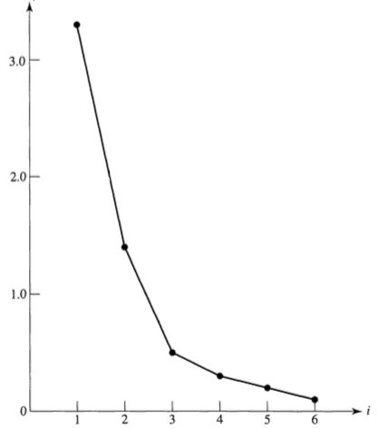
Total variance: $\sum_{j=1}^n \lambda_j^2$.

Scree plot: choose the number of principal components by the elbow method.

Reduced Rank Approximation by SVD

From SVD:

\[\frac{1}{\sqrt{m}}X = U \Sigma V^T = \sum_{j=1}^n \lambda_j u_j v_j^T\]

Let $s < n = \text{rank}(X)$. The reduced rank-$s$ least-squares approximation is

\[\frac{1}{\sqrt{m}}\widehat{X} = \sum_{j=1}^s \lambda_j u_j v_j^T\]

which minimizes the Frobenius norm

\[\frac{1}{m} \sum_{i=1}^m \sum_{j=1}^n \left( x_{ij} - \widehat{x}_{ij} \right)^2 = \text{tr} \left[ \left(\frac{1}{\sqrt{m}} (X - \widehat{X}) \right) \left(\frac{1}{\sqrt{m}} (X - \widehat{X}) \right)^T \right]\]

over all matrices $\widehat{X}$ of rank no greater than $s$ (Eckart-Young theorem).

PCA Algorithm Summary

1. Standardize each feature: $x_j \leftarrow (x_j - \bar{x}_j)/\sigma_j$
2. Compute eigenvectors of $\Sigma_X = \frac{1}{m}X^TX$
3. The $i$-th principal component is $v_i$; its explained variance is $d_i$
4. Select number of components $s$ via scree plot (elbow on ${\lambda_j^2}$); total variance is $\sum_j \lambda_j^2$

Key Equation

\[\frac{1}{m}X^TX = VDV^T \quad \text{(eigendecomposition / PCA)}\] \[\frac{1}{\sqrt{m}}X = U\Sigma V^T \quad \text{(SVD)}\] \[\frac{1}{\sqrt{m}}\widehat{X} = \sum_{j=1}^s \lambda_j u_j v_j^T \quad \text{(rank-}s\text{ approximation, Eckart-Young)}\]

Analogy

PCA is like finding the natural axes of an ellipse fitted to a point cloud: the major axis captures the most spread (highest variance), the minor axis captures the least. SVD is the same operation written in terms of the data matrix directly rather than its covariance.

Component of

• Dimensionality Reduction #todo
• Singular Value Decomposition #todo

Insights

• SVD and PCA are two views of the same decomposition: $\lambda_j^2 = d_j$.
• Rank-$s$ SVD is the optimal least-squares approximation to $X$ (Eckart-Young theorem).
• PCA is scale-sensitive: normalization is mandatory before computing the covariance.

Pitfalls

• PCA assumes linear structure; nonlinear geometry requires Kernel PCA or manifold methods.
• PCA is sensitive to outliers since covariance is not robust.

Connections

• Correspondence Analysis: generalized SVD applied to categorical count data.
• Kernel PCA #todo
• Eckart-Young Theorem #todo

Implementation Notes

• Prefer np.linalg.svd over explicit eigendecomposition for numerical stability.
• For large $n$, use randomized SVD (e.g., sklearn.utils.extmath.randomized_svd) to avoid the $O(n^3)$ cost.

References

• Shlens (arXiv, 2014). A Tutorial on Principal Component Analysis.
• Johnson & Wichern (2002). Applied Multivariate Statistical Analysis.