A (Comprehensive) Look into Correspondence Analysis
Outline
- What is Correspondence Analysis?
- Why Correspondence Analysis?
- Methodology Summary
- Visualization Maps
- Numpy Implementations of Correspondence Analysiss
- References
What is Correspondence Analysis?
- Aggregate data based: more useful and convenient, compared with raw data-based.
- Dimension reduction: represent associations in a table of nonnegative counts.
- Data visualization for association: the positions of the points reflect associations.
Numerous applications
- Segments vs. Genders
- Segments vs. 24 hours
- Segments vs. 7 weekdays
- Segments vs. Locations
- Segments vs. App detection
- Segments vs. {only-impressions, with-clicks and further-with-actions}
- Campaigns vs. {only-impressions, with-clicks and further-with-actions}
- Other groups vs. characteristics, etc…
Correspondence analysis of archaeological data: sites vs. types
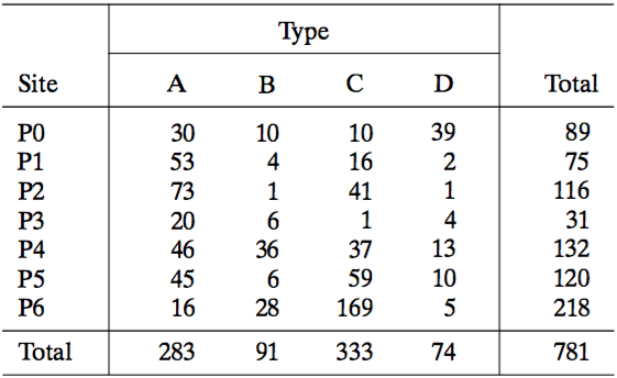
Common data visualizations:
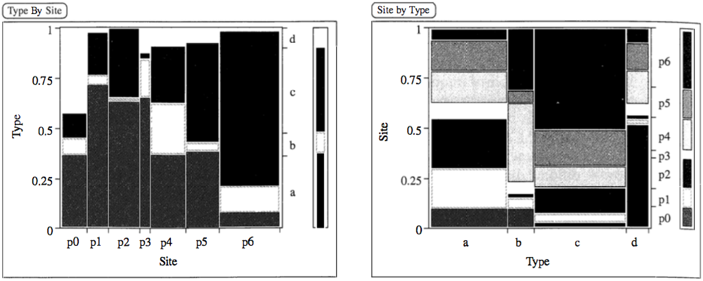
However, common data visualizations of type by site (left) and site by type (right) cannot quantify associations.
Correspondence analysis vidualization:
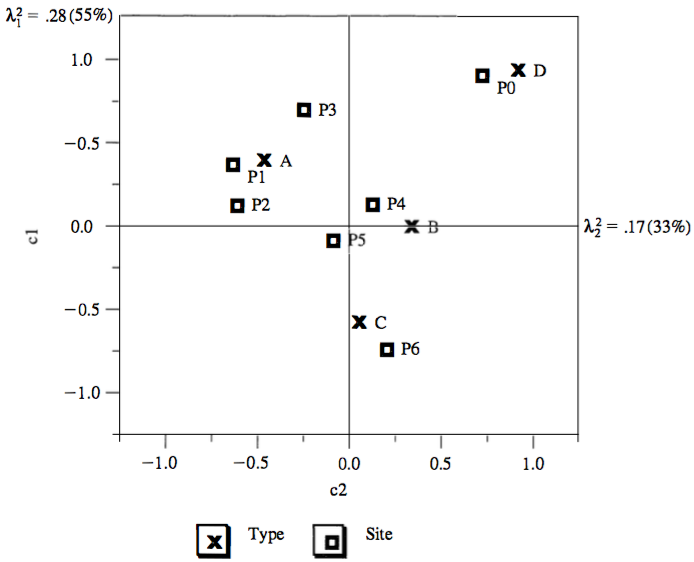
- Sites association:
- P1 and P2 are close together, and thus have similar type profiles
- P0 ad P6 are far apart, and thus have different type profiles
- Types association:
- A, B, C and D have different site profiles
- Site and type association: (rough, see later)
- Site P0 is associated almost exclusively with type D
- Site P6 is similarly associated with type C
- Sites P1, P2 and P3 (to lesser degrees) are associated with type A
- Measure of retained information:
- Inertia: amount of retained information with
- 1st dimension: \(\lambda^2_1 = 0.28 (55\%)\)
- 2nd dimension: \(\lambda^2_2 = 0.17 (28\%)\)
- The two dimensions account for \(55\% + 28\% = 88\%\) of the total inertia
- The representations fits the data well
- Inertia: amount of retained information with
Why Correspondence Analysis?
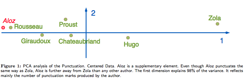
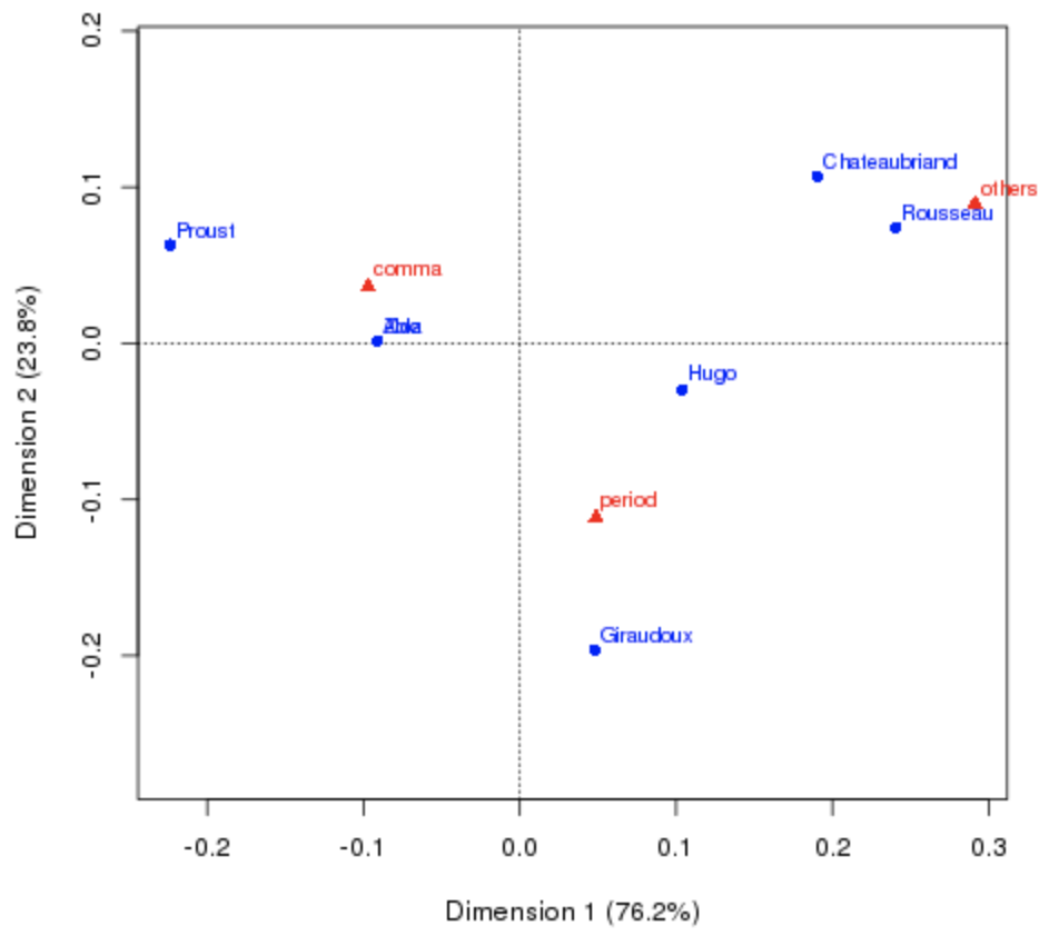
French authors dataset:
- Goal: Derive a map that reveals the similarities in punctuation style between authors.
- Note: Zola, who wrote a small novel under a pseudonym of Aloz.
from __future__ import division
from __future__ import print_function

import numpy as np
import scipy as sp
import pandas as pd
data = {'period': [7836, 53655, 115615, 161926, 38177, 46371, 2699],
        'comma': [13112, 102383, 184541, 340479, 105101, 58367, 5675],
        'others': [6026, 42413, 59226, 62754, 12670, 14299, 1046]}
data = pd.DataFrame(data, columns=['period', 'comma', 'others'],
                    index=['Rousseau', 'Chateaubriand', 'Hugo', \
                           'Zola', 'Proust', 'Giraudoux', 'Aloz'])
data
| period | comma | others | |
|---|---|---|---|
| Rousseau | 7836 | 13112 | 6026 |
| Chateaubriand | 53655 | 102383 | 42413 |
| Hugo | 115615 | 184541 | 59226 |
| Zola | 161926 | 340479 | 62754 |
| Proust | 38177 | 105101 | 12670 |
| Giraudoux | 46371 | 58367 | 14299 |
| Aloz | 2699 | 5675 | 1046 |
First (bad) idea: PCA (sometimes)
- Aloz punctuates the style similarity as Zola, but is farther away from Zola than any authors.
- That is because PCA is mainly sensitive to the number of produced punctuation marks.
Correspondence analysis is successful:
- From correspondence analysis results, Aloz and Zola are close together!
- It successfully reveals profile (style) similarity.
Methodology Summary
Correspondence Analysis is based on generalized singular value decomposition (SVD), which is similar to principal component analysis (PCA), except that the former applies to categorical rather than continuous data; for introduction to PCA and SVD, see my post.
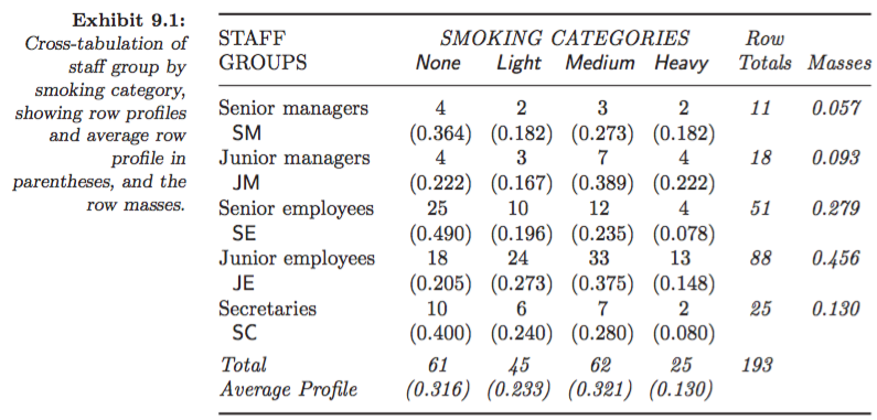
- Let the observed data be a contigency table of unscaled counts which is summarized data,
- The rows and columns of \(X\) correspond to different categories (groups) of different characteristics.
Define:
- Correspondence matrix: divide \(x_{ij}\) by total count, \(n = \textstyle \sum_{i=1}^I \sum_{j=1}^J x_{ij}\), to obtain
- Row and column profiles:
\(r_i = \sum_{j=1}^J p_{ij} = \frac{1}{n} \sum_{j=1}^J x_{ij}, or \underset{I \times 1} r = P \mathbf{1}_J\) \(c_j = \sum_{i=1}^I p_{ij} = \frac{1}{n} \sum_{i=1}^I x_{ij}, or \underset{J \times 1} c = P^T \mathbf{1}_I\)
- Diagonal matrices with elements of \(r\) and \(c\):
\(D_r = diag(r_1,...,r_I)\) \(D_c = diag(c_1,...,c_J)\)
Correspondence analysis:
- It can be formulated as the reduced rank-K “weighted” least squares approximation to select \(\widehat{P} = \{p_{ij}\}\) which minimizes
- Result from (Johnson & Wichern, 2002, p. 72): The term \(r c^T\) is common to the approximation \(\widehat{P}\) whatever the correspondence matrix \(P\).
- Thus, it is equivalent to minimize
- Similarly with SVD, compute the SVD of \(D_r^{-1/2} (P - r c^T) D_c^{-1/2}\):
where \(U\) and \(V\) are orthogonal matrices with \(U^T U = V^T V = I\), and \(\Sigma\) is a rank-K diagonal matrix.
- Thus,
where \(A = D_r^{1/2} U\) and \(B = D_c^{1/2} V\).
- The above decomposition is often called generalized SVD:
- Row profile matrix: divide each row by its sum,
- Column profile matrix: divide each column by its sum,
- Row deviations from average row profile:
- Column deviations from average column profile: similarly,
Hence, we can obtain coordinates of the row and column profiles:
- Principal coordinates of rows: The coordinates for \((R - \mathbf{1}_I c^T)\) w.r.t. the axes of \(b_1,...,b_J\) are given by the columns of
- Principal coordinates of columns: The coordinates for \((C - r\mathbf{1}_J^T)^T\) w.r.t. the axes of \(a_1,...,a_I\) are given by the columns of
- Standard coordinates of rows:
- Standard coordinates of columns:
- Relationship:
\(F^T D_r F = G^T D_c G = \Sigma^2\) \(\Phi^T D_r \Phi = \Gamma^T D_c \Gamma = I\)
Inertia: total variance of the correspondence matrix \(P\), which resembles a chi-square statistic,
\[Inertia = \sum_{i=1}^I \sum_{j=1}^J \frac{\left( p_{ij} - r_i c_j \right)^2}{r_i c_j} = \sum_{k=1}^K \lambda_k^2\]Evaluation of 2D graphical display:
- Inertia associated with dimension \(k\), for \(k = 1,2\): \(\lambda_k^2\).
- Proportion of total inertia: explained total variance; the larger, the better.
Visualization Maps
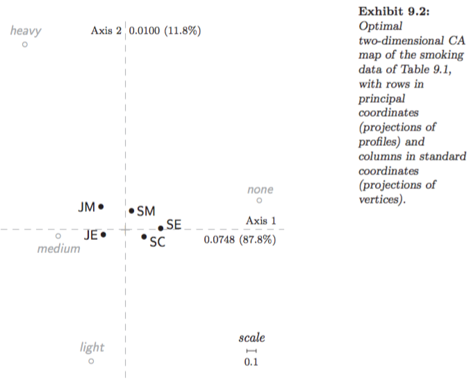
- (1) Symmetric map: \((F, G)\), rows and columns in principal coordinates.
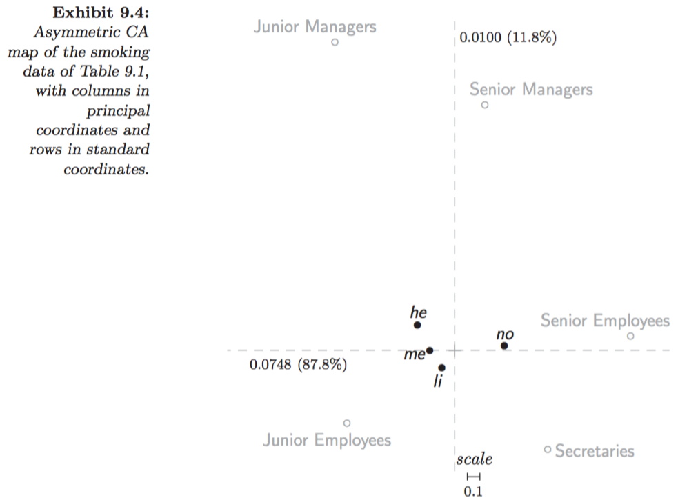
- (2) Asymmetric map with row principal: \((F, \Gamma)\), rows (of more interest) in principal and columns in standard coordinates.
- (3) Asymmetric map with column principal: \((\Phi, G)\), rows in standard and columns (of more interest) in principal corordinates.
For interpretation details please see (Greenacre, 2007, p. 66 - 72).
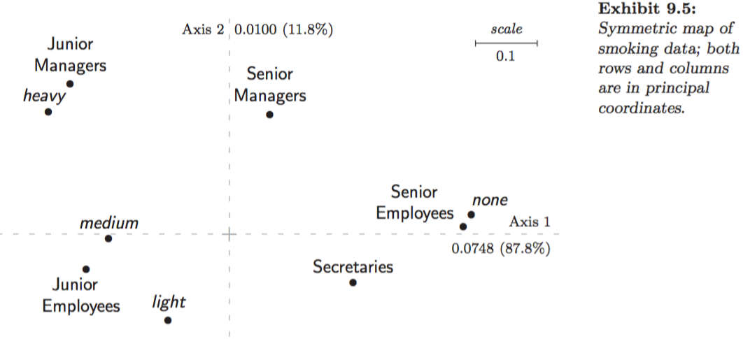
Symmetric map (1):
- Since principal coordinates of rows and columns, \((F, G)\), are scaled similarly, joint display of two separate maps finds some justification.
- Thus, row-to-row distance interpretation (and column-to-column distance interpretation) are meaningful.
- However, there is a danger in row-to-column distance interpretation: not possible to deduce from the closeness of a row and column point the fact that the corresponding row and column necessarily have a high association, since the row space and column space are different.
Asymmetric maps (2) and (3):
- Notice that the row and column points in biplot lie in the same space (why? since \(F\) is with respect to basis \(B\), and \(\Gamma B^T = I\)), thus not only row-to-row and column-to-column distance interpretations, but also row-to-column distance interpretation are meaningful.
- Hence, closeness of a row and column point indicates a high association; we can calculate row-to-column distances for one column at a time.
Interpretations:
- Asymmetric plots allow us to intuitively interpret the row-to-row, column-to-column, and row-to-column distances, especially if the first two components have a large proportion of the total inertia.
- However, the principal points on an asymmetric plot might appear too close to each other in the center of the map, which makes the graph difficult to view. In the case, we may also display a symmetric plot to more clearly view the relationships among either the row or column categories.
Example: Smoking dataset:
Figures 9.2 in Greenacre (2007):
Figures 9.4 in Greenacre (2007):
Figures 9.5 in Greenacre (2007):
Numpy Implementations of Correspondence Analysis
# https://github.com/bowen0701/machine-learning/blob/master/correspondence_analysis.py
from __future__ import absolute_import
from __future__ import division
from __future__ import print_function

import numpy as np
import scipy as sp
import pandas as pd
from numpy.linalg import svd

class CorrespondenceAnalysis(object):
    """Correspondence analysis (CA).

    Methods:
      fit: Fit correspondence analysis.
      get_coordinates: Get symmetric or asymmetric map coordinates.
      score_inertia: Get score inertia.

    ### Usage
    corranal = CA(aggregate_cnt)
    corranal.fit()
    coord_df = corranal.get_coordinates()
    inertia_prop = corranal.score_inertia()
    """

    def __init__(self, df):
        """Create a new Correspondence Analysis.

        Args:
          df: Pandas DataFrame, with row and column names.

        Raises:
          TypeError: Input data  is not a pandas DataFrame
          ValueError: Input data  contains missing values.
          TypeError: Input data  contains data types other than numeric.
        """
        if isinstance(df, pd.DataFrame) is not True:
            raise TypeError('Input data is not a Pandas DataFrame.')
        self._rows = np.array(df.index)
        self._cols = np.array(df.columns)
        self._np_data = np.array(df.values)
        if np.isnan(self._np_data).any():
            raise ValueError('Input data contains missing values.')
        if np.issubdtype(self._np_data.dtype, np.number) is not True:
            raise TypeError('Input data contains data types other than numeric.')

    def fit(self):
        """Compute Correspondence Analysis.

        Fit method is to
          - perform generalized singular value decomposition (SVD) for
            correspondence matrix and
          - compute principal and standard coordinates for rows and columns.

        Returns:
          self: Object.
        """
        p_corrmat = self._np_data / self._np_data.sum()
        r_profile = p_corrmat.sum(axis=1).reshape(p_corrmat.shape[0], 1)
        c_profile = p_corrmat.sum(axis=0).reshape(p_corrmat.shape[1], 1)
        Dr_invsqrt = np.diag(np.power(r_profile, -1/2).T[0])
        Dc_invsqrt = np.diag(np.power(c_profile, -1/2).T[0])
        ker_mat = np.subtract(p_corrmat, np.dot(r_profile, c_profile.T))
        left_mat = Dr_invsqrt
        right_mat = Dc_invsqrt
        weighted_lse = left_mat.dot(ker_mat).dot(right_mat)
        U, sv, Vt = svd(weighted_lse, full_matrices=False)
        self._Dr_invsqrt = Dr_invsqrt
        self._Dc_invsqrt = Dc_invsqrt
        self._U = U
        self._V = Vt.T
        self._SV = np.diag(sv)
        self._inertia = np.power(sv, 2)
        # Pricipal coordinates for rows and columns.
        self._F = self._Dr_invsqrt.dot(self._U).dot(self._SV)
        self._G = self._Dc_invsqrt.dot(self._V).dot(self._SV)
        # Standard coordinates for rows and columns.
        self._Phi = self._Dr_invsqrt.dot(self._U)
        self._Gam = self._Dc_invsqrt.dot(self._V)
        return self

    def _coordinates_df(self, array_x1, array_x2):
        """Create pandas DataFrame with coordinates in rows and columns.

        Args:
          array_x1: numpy array, coordinates in rows.
          array_x2: numpy array, coordinates in columns.

        Returns:
          coord_df: A Pandas DataFrame with columns
            {'x_1',..., 'x_K', 'point', 'coord'}:
            - x_k, k=1,...,K: K-dimensional coordinates.
            - point: row and column points for labeling.
            - coord: {'row', 'col'}, indicates row point or column point.
        """
        row_df = pd.DataFrame(
            array_x1,
            columns=['x' +  str(i) for i in (np.arange(array_x1.shape[1]) + 1)])
        row_df['point'] = self._rows
        row_df['coord'] = 'row'
        col_df = pd.DataFrame(
            array_x2,
            columns=['x' +  str(i) for i in (np.arange(array_x2.shape[1]) + 1)])
        col_df['point'] = self._cols
        col_df['coord'] = 'col'
        coord_df = pd.concat([row_df, col_df], ignore_index=True)
        return coord_df

    def get_coordinates(self, option='symmetric'):
        """Take coordinates in rows and columns for symmetric or assymetric map.

        For symmetric vs. asymmetric map:
          - For symmetric map, we can catch row-to-row and column-to-column
            association (maybe not row-to-column association);
          - For asymmetric map, we can further catch row-to-column association.

        Args:
          option: string, in one of the following three:
            'symmetric': symmetric map with
              - rows and columns in principal coordinates.
            'rowprincipal': asymmetric map with
              - rows in principal coordinates and
              - columns in standard coordinates.
            'colprincipal': asymmetric map with
              - rows in standard coordinates and
              - columns in principal coordinates.

        Returns:
          Pandas DataFrame, contains coordinates, row and column points.

        Raises:
          ValueError: Option only includes {"symmetric", "rowprincipal", "colprincipal"}.
        """
        if option == 'symmetric':
            # Symmetric map
            return self._coordinates_df(self._F, self._G)
        elif option == 'rowprincipal':
            # Row principal asymmetric map
            return self._coordinates_df(self._F, self._Gam)
        elif option == 'colprincipal':
            # Column principal asymmetric map
            return self._coordinates_df(self._Phi, self._G)
        else:
            raise ValueError(
                'Option only includes {"symmetric", "rowprincipal", "colprincipal"}.')

    def score_inertia(self):
        """Score inertia.

        Returns:
          A NumPy array, contains proportions of total inertia explained
            in coordinate dimensions.
        """
        inertia = self._inertia
        inertia_prop = (inertia / inertia.sum()).cumsum()
        return inertia_prop
Cited as:
@article{li2016pcasvd,
  title   = "A (Comprehensive) Look into Correspondence Analysis",
  author  = "Li, Bowen",
  journal = "https://bowen0701.github.io/",
  year    = "2016",
  url     = "https://bowen0701.github.io/2016/10/06/correspondence-analysis/"
}
If you notice errors in this post, please contact me at [bowen0701 at gmail dot com] and I would be grateful to be able to correct them.
See you in the next post. :-)
References
[1] Johnson & Wichern (2002). Applied Multivariate Statistical Analysis.
[2] Nenadic & Greenacre (JSS, 2007). Correspondence Analysis in R, with Two- and Three-dimensional Graphics: The ca Package.
[3] Greenacre (2007). Correspondence Analysis in Practice.
[4] Greenacre (2010). Biplots in Practice.