A (Detailed) Peek into PCA and SVD

Outline

• What is Principal Component Analysis (PCA)?
  • Assumptions for PCA
  • Eigendecomposition
  • Summary of PCA
• What is Singular Value Decomposition (SVD)?
  • Matrix Version of SVD
• PCA and SVD
  • How Many Pricipal Components We Shall Use?
  • Reduced Rank Approximation by SVD
• References

What is PCA?

The motivation of PCA is to identify the most meaningful basis to re-express data which can maximize the signal-to-noise ratio (SNR): \(\sigma^2_{signal} / \sigma^2_{noise}\).

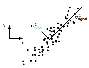
• Maximize the signal, measured by the magnitude of variance; large variance corresponds to interesting structure.
• Minimize redundancy (i.e. noise), measured by the magnitude of covariance.

Let the observed data be

where each row, \(x^T_{i.}\), represents an example measured on \(n\)-dimensional features,

and each column, \(x_{.j}\), represents normalized feature with zero means, \(E(x_{.j}) = 0\), and variance one, \(Var(x_{.j}) = 1\).

For notation simplicity, we also denote each row \(x^T_{i.}\) by \(x^T_i\).

The covariance matrix of \(X\) is

Our goal is to find some transformation, \(Y = f(X)\), of X such that covariance of \(Y\) is a diagonal matrix,

There are many transformations for diagonalizing the convariance matrix \(\Sigma_X\), PCA arguably selects the easiest one.

Assumptions for PCA

• Linear transformation: Let \(\underset{n \times n}E = [e_1,...,e_n]\),

• Large variance have important structure.
• The principal components are orthogonal.

The last assumption provides an intuitive simplification that makes PCA soluble with linear algebra decomposition techniques.

Eigendecomposition

The eigendecomposition, or eigenvector decomposition, is also called the spectral secomposition. Suppose \(Y = XE\), its covariance matrix

Since \(\frac{1}{m}X^TX\) is a symmetric matrix, it can be diagonalized by a matrix of orthonormal eigenvectors using the spectral decomposistion,

where \(D = diag(d_1,...,d_n)\) is a diagonal matrix with rank-ordered set of eigenvalues, \(d_1 \ge d_2 \ge ... \ge d_n\), and \(V = [v_1,...,v_n]\) is the matrix of the corresponding eigenvectors with \(V^TV=VV^T = I\).

Sketch of proof: From the spectral decomposition, for all \(j\), we have

Then we have \(\frac{1}{m}X^T X V = V D\) which implies \(\frac{1}{m}X^T X = V D V^T\).

Alternative proof: We can interpret PCA as finding a unit vector \(u\), with \(\|u\| = 1\), which maximizes variance of the projection of all example \(x_i\)’s onto \(u\),

But let’s digress a little to ask why the variance of the projection of all examples \(x_i\) onto \(u\) has form like the above? First, suppose the angle between \(x_i\) and \(u\) is \(\theta\), then the projection of each example \(x_i\) onto \(u\) is

since \(u\) is a unit vector. Then the length of the projection of one example \(x_i\) onto \(u\) is

since \(x_i^T x_i = \|x_i\|^2\). Finally, the projection of one example \(x_i\)’s onto \(u\) is the distance \(x_i^T u\) from the origin.

Now let’s go back to our optimization problem, we would like to solve

such that \(u^T u = 1\). Using the lagrange multiplier method, the objective becomes

Take partial derivative with respect to \(u\) we have

Hence, we are solving \(\frac{1}{m} X^T X u = d u\), and the eigenvector decomposition result follows.

From the above results we can select \(E = V\). Then since \(V^TV=VV^T = I\), \(\Sigma_Y\) now is a diagonal matrix

Note that the eigenvalue \(d_j\) is the variance of transformed feature \(y_j\).

Summary of PCA

• Substract off the mean of each feature: \(x_j \leftarrow x_j - \overline x_j\), and divide the standard deviation: \(x_j \leftarrow x_j/\sigma_j\)
• Compute the eigenvectors of covariance matrix, \(\Sigma_X = \frac{1}{m}X^TX\)
• The ith principal components of \(X\) is the covariance matrix \(\Sigma_X\)’s eigenvector \(v_i\)
• The ith diagonal value of the transformed covariance matrix \(\Sigma_Y\) is the variance of \(X\) along \(v_i\)

What is SVD?

First recall the eigenvector decomposition: \(\frac{1}{m}X^T X v_j = d_j v_j\). Define

• Singular values: square root of eigenvalue (variance) \(\lambda_j = \sqrt{d_j}\), for \(j = 1,...,n\).
• Matrix \(U = [ u_1,...,u_n ]\), with \(u_j\) defined by

where \(v_j\) is the eigenvector.

Then we have

• (1) \(U\) is orthonormal matrix: \(u_i^T u_j = \begin{cases} 1, \text{if } i = j \\ 0, \text{otherwise} \end{cases}\)
• (2) \(\lVert X v_i\rVert = \lambda_i\)

Sketch of proof: \(u_i^T u_j = \frac{1}{m} \left( \frac{1}{\lambda_i} X v_i \right)^T \left( \frac{1}{\lambda_j} X v_j \right) = \frac{1}{\lambda_i \lambda_j} v_i^T \frac{1}{m} X^T X v_j = \frac{1}{\lambda_i \lambda_j} v_i^T d_j v_j = \frac{\lambda_j}{\lambda_i} v_i^T v_j\). The first result follows. Further, we can obtain the second result similarly.

By rewriting we have

That is, normalized \(X\) multiplied by an eigenvector \(v_j\) of covariance of \(X\), \(\frac{1}{m} X^T X\), is equal to a scalar \(\lambda_j\) times another vector, \(u_j\).

Matrix Version of SVD

• By constructing a new diagonal matrix of singular values, \(\Sigma = diag(\lambda_1,...,\lambda_n)\), where \(\lambda_1 \ge \lambda_2 \ge ... \ge \lambda_n\).
• Define \(V = [v_1,...,v_n]\) and \(U = [u_1,...,u_n]\).

Hence, any arbitrary matrix \(\frac{1}{\sqrt{m}}X\) can be transformed to

• an orthogonal matrix (rotation): \(U\)
• a diagonal matrix (stretch): \(\Sigma\)
• another orthogonal matrix (second rotation): \(V\)

PCA and SVD

From SVD, we have

That is, squared singular value is equal to variance of \(X\) along eigenvector \(v_j\), \(\lambda_j^2 = d_j\).

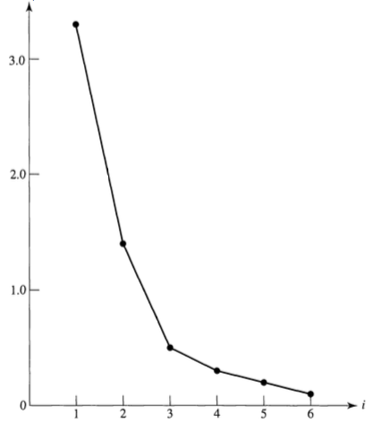
How Many Pricipal Components We Shall Use?

• Total variances: \(\sum_{j=1}^n \lambda_j^2\).
• Scree plot: Choose the number of principal component by elbow method.

Reduced Rank Approximation by SVD

Recall from SVD,

Let \(s < n = rank(X)\). Then the reduced rank-\(s\) least squares approximation to \(\frac{1}{\sqrt{m}} X\) is

which minimizes the Frobenius norm,

over all matrices \(\widehat{X}\) having rank no greater than \(s\). This optimization problem can be solved using eigendecomposition as above.

Cited as:

@article{li2016pcasvd,
  title   = "A (Detailed) Peek into PCA and SVD",
  author  = "Li, Bowen",
  journal = "https://bowen0701.github.io/",
  year    = "2016",
  url     = "https://bowen0701.github.io/2016/10/05/pca-svd/"
}

If you notice errors in this post, please contact me at [bowen0701 at gmail dot com] and I would be grateful to be able to correct them.

See you in the next post. :-)

References

[1] Shlens (arXiv, 2014). A Tutorial on Principal Component Analysis.

[2] Johnson & Wichern (2002). Applied Multivariate Statistical Analysis.## References